Our World in Data’dan veri indirme#
Our World in Data yakın zamanda verilerine erişim için API’ler sağladığını duyurdu. Rastlantı eseri veri kümelerinden birini PyData Global 2024 zaman serisi analizi atölyemde kullanıyorum. Örneğimi yeni API ile güncelledim; bu notebook öğrendiklerimi gösteriyor.
Bu notebook’u Colab’da çalıştırmak için buraya tıklayın. Think Stats, üçüncü baskının 12. bölümüne dayanır.
import numpy as np
import pandas as pd
import matplotlib.pyplot as plt
Hava sıcaklığı#
Zaman serisi analizi bölümündeki mevsimsel ayrıştırma alıştırmasında, Our World in Data’nın 1941–2024 arasında çoğu ülke için “kara, deniz ve iç su yüzeylerini kapsayan, yerden 2 metre yüksekte ölçülmüş hava sıcaklığını [Santigrat]” içeren veri kümesinden ABD aylık ortalama yüzey sıcaklıklarını kullanıyorum.
Aşağıdaki hücreler veri kümesini açıklayan metadata’yı indirip gösterir.
import requests

url = (
    "https://ourworldindata.org/grapher/"
    "average-monthly-surface-temperature.metadata.json"
)
query_params = {"v": "1", "csvType": "full", "useColumnShortNames": "true"}
headers = {"User-Agent": "Our World In Data data fetch/1.0"}

response = requests.get(url, params=query_params, headers=headers)
metadata = response.json()
Sonuç iç içe sözlüktür. Üst düzey anahtarlar şöyledir.
metadata.keys()
dict_keys(['chart', 'columns', 'dateDownloaded'])
Grafik düzeyindeki belgeleme şöyledir.
from pprint import pprint

pprint(metadata["chart"])
{'citation': 'Contains modified Copernicus Climate Change Service information '
             '(2019)',
 'originalChartUrl': 'https://ourworldindata.org/grapher/average-monthly-surface-temperature?v=1&csvType=full&useColumnShortNames=true',
 'selection': ['World'],
 'subtitle': 'The temperature of the air measured 2 meters above the ground, '
             'encompassing land, sea, and in-land water surfaces.',
 'title': 'Average monthly surface temperature'}
Kullanacağımız sütunun belgelemesi şöyledir.
pprint(metadata["columns"]["temperature_2m"])
{'citationLong': 'Contains modified Copernicus Climate Change Service '
                 'information (2019) – with major processing by Our World in '
                 'Data. “Annual average” [dataset]. Contains modified '
                 'Copernicus Climate Change Service information, “ERA5 monthly '
                 'averaged data on single levels from 1940 to present 2” '
                 '[original data].',
 'citationShort': 'Contains modified Copernicus Climate Change Service '
                  'information (2019) – with major processing by Our World in '
                  'Data',
 'descriptionKey': [],
 'descriptionProcessing': '- Temperature measured in kelvin was converted to '
                          'degrees Celsius (°C) by subtracting 273.15.\n'
                          '\n'
                          '- Initially, the temperature dataset is provided '
                          'with specific coordinates in terms of longitude and '
                          'latitude. To tailor this data to each country, we '
                          'utilize geographical boundaries as defined by the '
                          'World Bank. The method involves trimming the global '
                          'temperature dataset to match the exact geographical '
                          'shape of each country. To correct for potential '
                          "distortions caused by the Earth's curvature on a "
                          'flat map, we apply a latitude-based weighting. This '
                          'step is essential for maintaining accuracy, '
                          'especially in high-latitude regions where '
                          'distortion is more pronounced. The result of this '
                          'process is a latitude-weighted average temperature '
                          'for each nation.\n'
                          '\n'
                          "- It's important to note, however, that due to the "
                          'resolution constraints of the Copernicus dataset, '
                          'this methodology might not be as effective for '
                          'countries with very small landmasses. In these '
                          'cases, the process may not yield reliable data.\n'
                          '\n'
                          '- The derived 2-meter temperature readings for each '
                          'country are calculated based on administrative '
                          'borders, encompassing all land surface types within '
                          'these defined areas. As a result, temperatures over '
                          'oceans and seas are not included in these averages, '
                          'focusing the data primarily on terrestrial '
                          'environments.\n'
                          '\n'
                          '- Global temperature averages and anomalies are '
                          'calculated over all land and ocean surfaces.',
 'descriptionShort': 'The temperature of the air measured 2 meters above the '
                     'ground, encompassing land, sea, and in-land water '
                     'surfaces. The 2024 data is incomplete and was last '
                     'updated 13 October 2024.',
 'fullMetadata': 'https://api.ourworldindata.org/v1/indicators/819532.metadata.json',
 'lastUpdated': '2023-12-20',
 'owidVariableId': 819532,
 'shortName': 'temperature_2m',
 'shortUnit': '°C',
 'timespan': '1940-2024',
 'titleLong': 'Annual average',
 'titleShort': 'Annual average',
 'type': 'Numeric',
 'unit': '°C'}
Aşağıdaki hücreler ABD verilerini indirir. Başka ülke için country_code değerini hemen her üç harfli ISO 3166 ülke koduyla değiştirebilirsiniz.
country_code = "USA"  # başka üç harfli ülke kodlarıyla değiştirilebilir
base_url = (
    "https://ourworldindata.org/grapher/"
    "average-monthly-surface-temperature.csv"
)

query_params = {
    "v": "1",
    "csvType": "filtered",
    "useColumnShortNames": "true",
    "tab": "chart",
    "country": country_code,
}
from urllib.parse import urlencode

url = f"{base_url}?{urlencode(query_params)}"
temp_df = pd.read_csv(url, storage_options=headers)
Desteklenen sorgu parametrelerini genellikle veri kümesini çevrimiçi inceleyip indirme simgesine basarak görebilirsiniz; görüntülenen URL, grafik üzerinde seçtiğiniz süzgeçlere karşılık gelen sorgu parametrelerini içerir.
temp_df.head()
| Entity | Code | year | Day | temperature_2m | temperature_2m.1 | |
|---|---|---|---|---|---|---|
| 0 | United States | USA | 1941 | 1941-12-15 | -1.878019 | 8.016244 |
| 1 | United States | USA | 1942 | 1942-01-15 | -4.776551 | 7.848984 |
| 2 | United States | USA | 1942 | 1942-02-15 | -3.870868 | 7.848984 |
| 3 | United States | USA | 1942 | 1942-03-15 | 0.097811 | 7.848984 |
| 4 | United States | USA | 1942 | 1942-04-15 | 7.537291 | 7.848984 |
Oluşan DataFrame, metadata’da belgelenen temperature_2m sütununu ve yıllık ortalama olabilecek belgelenmemiş ek sütunu içerir.
Bu örnekte aylık verileri kullanacağız.
temp_series = temp_df['temperature_2m']
temp_series.index = pd.to_datetime(temp_df['Day'])
Şöyle görünür.
temp_series.plot(label=country_code)
plt.ylabel("Surface temperature (℃)");
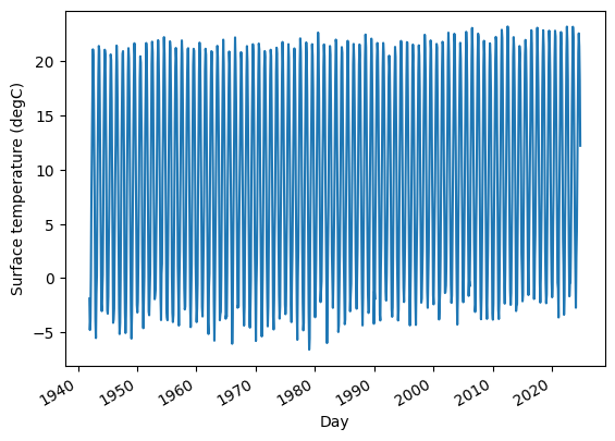
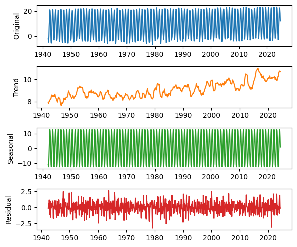
Şaşırtıcı olmayacak biçimde güçlü bir mevsimsel örüntü vardır. Uzun dönemli eğilim, mevsimsel bileşen ve artığı belirlemek için StatsModels içindeki seasonal_decompose işlevini kullanabiliriz.
from statsmodels.tsa.seasonal import seasonal_decompose

decomposition = seasonal_decompose(temp_series, model="additive", period=12)
Sonuçları çizmek için aşağıdaki işlevi kullanacağız.
def plot_decomposition(original, decomposition):
    plt.figure(figsize=(6, 5))

    plt.subplot(4, 1, 1)
    plt.plot(original, label="Özgün", color="C0")
    plt.ylabel("Özgün")

    plt.subplot(4, 1, 2)
    plt.plot(decomposition.trend, label="Eğilim", color="C1")
    plt.ylabel("Eğilim")

    plt.subplot(4, 1, 3)
    plt.plot(decomposition.seasonal, label="Mevsimsel", color="C2")
    plt.ylabel("Mevsimsel")

    plt.subplot(4, 1, 4)
    plt.plot(decomposition.resid, label="Artık", color="C3")
    plt.ylabel("Artık")

    plt.tight_layout()
plot_decomposition(temp_series, decomposition)
Bu tür veri kümelerini erişime açtığı ve artık program aracılığıyla kullanmayı kolaylaştırdığı için Our World in Data’ya her zamanki gibi minnettarım.
Think Stats: Python ile Keşifsel Veri Analizi, 3. Baskı
Telif hakkı 2024 Allen B. Downey
Kod lisansı: MIT Lisansı
Metin lisansı: Creative Commons Atıf-Gayriticari-AynıLisanslaPaylaş 4.0 Uluslararası